Quickstart
Single output model emulation
Assume that we have two arrays, X and y. y is of size N, and it stores the N expensive model outputs that have been produced by running the model on the N input sets of M input parameters in X. We will try to emulate the model by learning from these two training sets:
gp = gp_emulator.GaussianProcess(inputs=X, targets=y)
Now, we need to actually do the training…
gp.learn_hyperparameters()
Once this process has been done, you’re free to use the emulator to predict the model output for an arbitrary test vector x_test (size M):
y_pred, y_sigma, y_grad = gp.predict (x_test, do_unc=True,
                                       do_grad=True)
In this case, y_pred is the model prediction, y_sigma is the variance associated with the prediction (the uncertainty) and y_grad is an approximation to the Jacobian of the model around x_test.
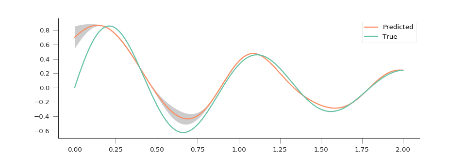
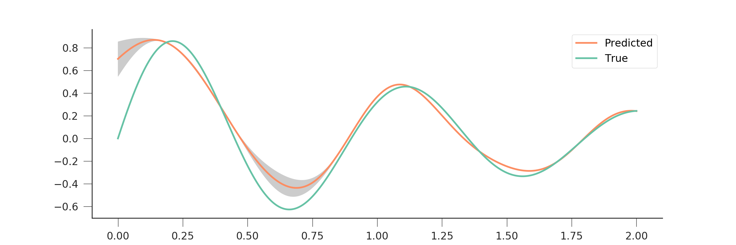
Let’s see a more concrete example. We create a damped sine, add a bit of Gaussian noise, and then subsample a few points (10 in this case), fit the GP, and predict the function over the entire range. We also plot the uncertainty from this prediction.
import numpy as np
import matplotlib.pyplot as plt

import gp_emulator

np.random.seed(42)
n_samples = 2000
x = np.linspace(0, 2, n_samples)
y = np.exp(-0.7*x)*np.sin(2*np.pi*x/0.9)
y += np.random.randn(n_samples)*0.02

# Select a few random samples from x and y
isel = np.random.choice(n_samples, 10)
x_train = np.atleast_2d(x[isel]).T
y_train = y[isel]
fig = plt.figure(figsize=(12,4))

gp = gp_emulator.GaussianProcess(x_train, y_train)
gp.learn_hyperparameters(n_tries=25)

y_pred, y_unc, _ = gp.predict(np.atleast_2d(x).T,
                                do_unc=True, do_deriv=False)
plt.plot(x, y_pred, '-', lw=2., label="Predicted")
plt.plot(x, np.exp(-0.7*x)*np.sin(2*np.pi*x/0.9), '-', label="True")
plt.fill_between(x, y_pred-1.96*y_unc,
                    y_pred+1.96*y_unc, color="0.8")
plt.legend(loc="best")
(Source code, png, hires.png, pdf)

We can see that the GP is doing an excellent job in predicting the function, even in the presence of noise, and with a handful of sample points. In situations where there is extrapolation, this is indicated by an increase in the predictive uncertainty.
Multiple output emulators
In some cases, we can emulate multiple outputs from a model. For example, hyperspectral data used in EO can be emulated by employing the SVD trick and emulating the individual principal component weights. Again, we use X and y. y is now of size N, P, and it stores the N expensive model outputs (size P) that have been produced by running the model on the N input sets of M input parameters in X. We will try to emulate the model by learning from these two training sets, but we need to select a variance level for the initial PCA (in this case, 99%)
gp = gp_emulator.MultivariateEmulator (X=y, y=X, thresh=0.99)
Now, we’re ready to use on a new point x_test as above:
y_pred, y_sigma, y_grad = gp.predict (x_test, do_unc=True,
                                        do_grad=True)
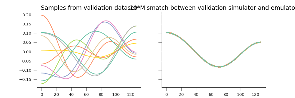
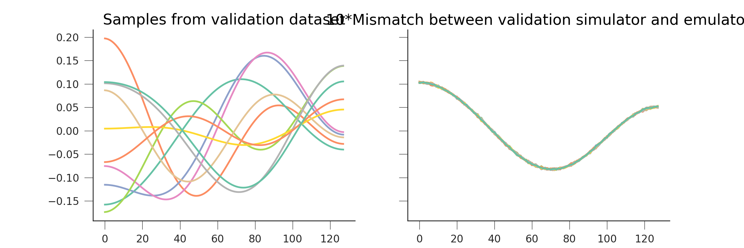
A more concrete example: let’s produce a signal that can be decomposed as a sum of scaled orthogonal basis functions…
import numpy as np

from scipy.fftpack import dct

import matplotlib.pyplot as plt
import gp_emulator


np.random.seed(1)

n_validate = 250
n_train = 100
basis_functions = dct(np.eye(128), norm="ortho")[:, 1:4]

params=["w1", "w2", "w3"]
mins = [-1, -1, -1]
maxs = [1, 1, 1]


train_weights, dists = gp_emulator.create_training_set(params, mins, maxs,
                                                        n_train=n_train)
validation_weights = gp_emulator.create_validation_set(dists,
                                                    n_validate=n_validate)

training_set = (train_weights@basis_functions.T).T

training_set += np.random.randn(*training_set.shape)*0.0005
validation_set = (validation_weights@basis_functions.T).T

gp = gp_emulator.MultivariateEmulator (y=train_weights, X=training_set.T,
                                        thresh=0.973, n_tries=25)
y_pred = np.array([gp.predict(validation_weights[i])[0]
                        for i in range(n_validate)])

fig, axs = plt.subplots(nrows=1, ncols=2,sharey=True,figsize=(12, 4))
axs[0].plot(validation_set[:, ::25])
axs[1].plot(10.*(y_pred.T - validation_set))
axs[0].set_title("Samples from validation dataset")
axs[1].set_title("10*Mismatch between validation simulator and emulator")
(Source code, png, hires.png, pdf)