Emulating a typical radiative transfer model

This package was designed to emulate radiatie transfer models. The process entails the following steps:

1. Decide on what input parameters are required
2. Decide their ranges
3. Generate a training input parameter set
4. Run the model for each element of the input training set and store the outputs
5. Pass the input and output training pairs to the library, and let it fit the hyperparameters

We can show how this works with an example of the PROSPECT+SAIL model.

Setting the input parameter ranges

We can set the parameter names and their ranges simply by having lists with minimum and maximum values. This assumes a uniformly-distributed parameter distribution between those two boundaries, but other distributions are possible (we never had any reason to try them though!). We additionally set up the SRFs and other variables that need to be defined here… We train the model on 250 samples and test on (say) 100. 100 validation samples is probably too few, but for the sake of not waiting too much… ;-)

from functools import partial

import numpy as np

import gp_emulator

import prosail

# Spectral band definition. Just a top hat, with start and
# end wavlengths as an example
b_min = np.array( [ 620., 841, 459, 545, 1230, 1628, 2105] )
b_max = np.array( [ 670., 876, 479, 565, 1250, 1652, 2155] )
wv = np.arange ( 400, 2501 )
passband = []

# Number of training and validation samples
n_train = 250
n_validate = 100
# Validation number is small, increase to a more realistic value
# if you want

# Define the parameter names and their ranges
# Note that we are working here in transformed coordinates...

# Define geometry. Each emulator is for one geometry
sza = 30.
vza = 0.
raa = 0. # in degrees

parameters = [ 'n', 'cab', 'car', 'cbrown', 'cw', 'cm', 'lai', 'ala', 'bsoil', 'psoil']
min_vals = [ 0.8       ,  0.46301307,  0.95122942,  0.        ,  0.02829699,
        0.03651617,  0.04978707,  0.44444444,  0.        ,  0.]
max_vals = [ 2.5       ,  0.998002  ,  1.        ,  1.        ,  0.80654144,
        0.84366482,  0.99501248,  0.55555556,  2.   , 1     ]

We then require a function for calling the RT model. In the case of PROSAIL, we can do that easily from Python, in other models available in e.g. Fortran, you could have a function that calls the external model

def inverse_transform ( x ):
    """Inverse transform the PROSAIL parameters"""
    x_out = x*1.
    # Cab, posn 1
    x_out[1] = -100.*np.log ( x[1] )
    # Cab, posn 2
    x_out[2] = -100.*np.log ( x[2] )
    # Cw, posn 4
    x_out[4] = (-1./50.)*np.log ( x[4] )
    #Cm, posn 5
    x_out[5] = (-1./100.)*np.log ( x[5] )
    # LAI, posn 6
    x_out[6] = -2.*np.log ( x[6] )
    # ALA, posn 7
    x_out[7] = 90.*x[7]
    return x_out



def rt_model ( x, passband=None, do_trans=True ):
    """A coupled land surface/atmospheric model, predicting refl from
    land surface parameters. Thisfunction provides estimates of refl for
    a particular illumination geometry.

    The underlying land surface reflectance spectra is simulated using
    PROSAIL. The input parameter ``x`` is a vector with the following components:

        * ``n``
        * ``cab``
        * ``car``
        * ``cbrown``
        * ``cw``
        * ``cm``
        * ``lai``
        * ``ala``
        * ``bsoil``
        * ``psoil``

    """
    x, sza, vza, raa = x

    # Invert parameter LAI
    if do_trans:
        x = inverse_transform ( x )
    ################# surface refl with prosail #####################

    surf_refl = prosail.run_prosail(x[0], x[1], x[2], x[3], x[4], x[5], x[6], x[7], 0.01, sza, vza, raa,
                    rsoil=x[8], psoil=x[9])
    if passband is None:
        return surf_refl
    else:
        return surf_refl[passband].mean()

Now we loop over all the bands, and prepare the emulators. we do this by using the create_emulator_validation function, that does everything you’d want to do… We just stuff the emulator, training and validation sets in one list for convenience.

retval = []
for iband,bmin in enumerate ( b_min ):
    # Looping over the bands....
    print("Doing band %d" % (iband+1))
    passband = np.nonzero( np.logical_and ( wv >= bmin, wv <= b_max[iband] ) )
    # Define the SRF for the current band
    # Define the simulator for convenience
    simulator = partial (rt_model, passband=passband)
    # Actually create the training and validation parameter sets, train the emulators
    # and return all that
    x = gp_emulator.create_emulator_validation (simulator, parameters, min_vals, max_vals,
                                n_train, n_validate, do_gradient=True,
                                n_tries=15, args=(30, 0, 0) )
    retval.append (x)

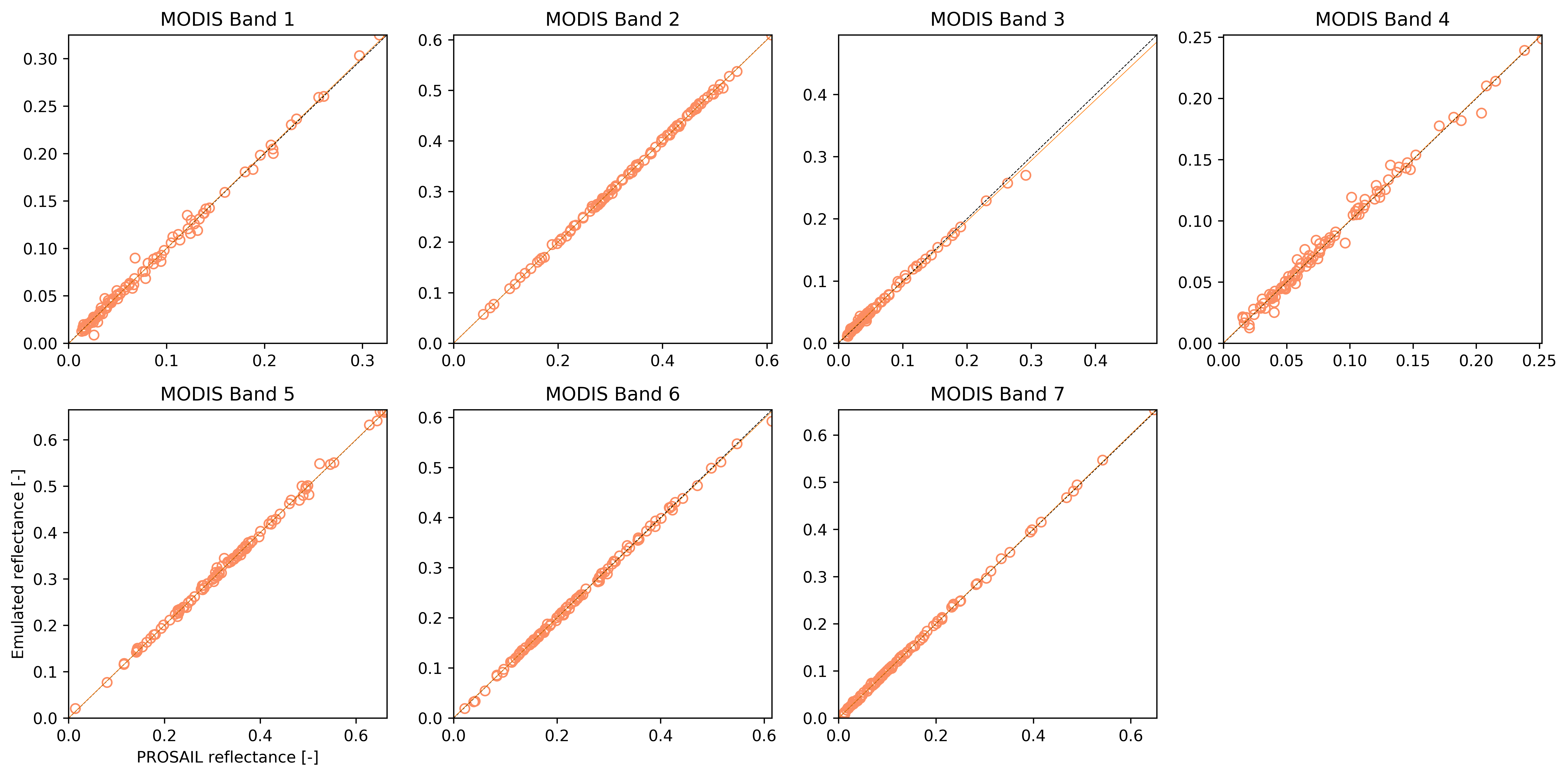
A simple validation visualisation looks like this

Comparison between the simulated output and the corresponding emulator output for the validation dataset. Correlations (R2) are in all cases better than 0.99. Slope was between 0.97 and 1., whereas the bias term was smaller than 0.002.

An spectral emulator of PROSAIL

For the case of a spectral emulator, the approach is the same, only that we just use the spectral emulator, which is a bit simpler.

n_train = 350
n_validate = 100
x = gp_emulator.create_emulator_validation ( rt_model, parameters, min_vals, max_vals,
                                n_train, n_validate, do_gradient=True,
                                n_tries=10, args=(30, 0, 0) )

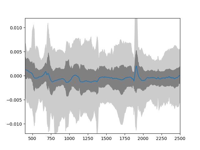
The validation results looks like this:

Distribution of residuals derived from the difference of the emulator and simulator for PROSAIL.

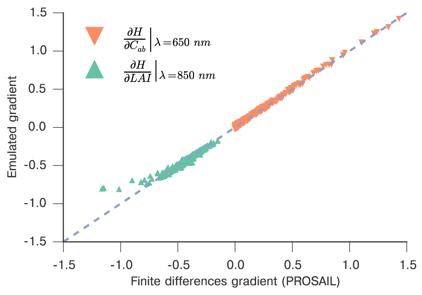
We can also check that the gradient of the model is sensible, by comparing it with finite difference approximations from the original model, which is already carried out by create_emulator_validation if we set the do_gradient option.

Comparison of the emulated model gradient versus finite difference approximation for LAI and chlorophyll at different spectral regions.